Search isn't magic, it's engineering. Understanding how it works will change how you build your search system.

In this article we'll build a simple keyword search implementation from scratch. You'll learn:

• What keyword search is
• How raw text becomes searchable data
• Why indexing is the secret to fast retrieval
• How BM25 ranking puts the most relevant results first (and why it beats simple word matching)

What is Keyword Search?

Keyword search is a method of finding documents by matching the exact words (or "keywords") that users type in their search queries. When you search for "machine learning," a keyword search system looks for documents that contain those specific terms.

Unlike semantic search systems that understand meaning and context, keyword search focuses on literal text matching. This makes it incredibly precise for exact terminology but less flexible for synonyms or conceptual queries.

For example, searching for "car" won't automatically return documents about "automobile" or "vehicle"—unless those exact words appear in the text.

Why Keyword Search Matters

Why is keyword important in the age of large language models, vector databases, and semantic search?

Consider these scenarios:

• Medical Search: A doctor searches for "COVID-19" and needs specific information about that exact condition, not a general collection of content about respiratory viruses or pandemic diseases.
• Financial Services: A compliance officer searches for "KYC requirements" (Know Your Customer) and needs regulatory documentation with this exact acronym, not general customer verification content
• Legal Research: A lawyer searches for "habeas corpus" and needs cases specifically invoking this writ, not general discussions about detention or constitutional rights

In each case, exact keyword matching is essential. The more technical and precise the terminology in your domain, the more powerful keyword search becomes.

Implementing Keyword Search

Let's dive into it. To implement it we need to cover 5 topics

1. Text Pre-Processing: Run, run, ran, runs all turn into run for keyword matching
2. Tokenization: Break text into individual words or terms
3. Indexing: For each word create a list of the documents that contain it
4. Matching: Find documents that contain the search terms
5. Ranking: Score and order results by relevance (typically using algorithms like BM25)

Text Processing

We need to clean up text so matching works reliably. Raw text doesn't work.

Cleaning Text

example_text = "Kubernetes orchestration enables efficient container management. The team implemented kubernetes clusters for high availability. They loved implementing kubernetes."

A search for "kubernetes" in the example text should match Kubernetes (capitalized), kubernetes (lowercase), and kubernetes.(punctuated).

Let's make that happen by making everything lowercase and removing punctuation.

import string

def clean_text(text):
    text = text.lower()
    text = text.translate(str.maketrans('', '', string.punctuation))
    return text

cleaned = clean_text(example_text)
print(cleaned)

kubernetes orchestration enables efficient container management the team implemented kubernetes clusters for high availability they loved implementing kubernetes

Now Kubernetes, kubernetes, and kubernetes. all become kubernetes.

Stemming and Lemmatization

Stemming reduces words to their root form. This helps "running", "runs", and "ran" all match "run".

Here's a simple stemmer:

def stem_text(text):
    words = text.split()
    
    stemmed = []
    for word in words:
        # Remove plural 's'
        if word.endswith('s') and len(word) > 3:
            word = word[:-1]
        
        # Remove 'ing'
        if word.endswith('ing'):
            word = word[:-3]
        
        # Remove 'ed'  
        if word.endswith('ed') and len(word) > 3:
            word = word[:-2]
            
        stemmed.append(word)
    
    return ' '.join(stemmed)

stemmed = stem_text(clean_text(example_text))
print(stemmed)

kubernete orchestration enable efficient container management the team implement kubernete cluster for high availability they lov implement kubernete

Now implemented and implementing both become implement.

def pre_process_text(text):
    "Clean and stem text"
    return stem_text(clean_text(text))

N-grams

So far we've been treating each word as an individual token (called "unigrams"). But sometimes the most important information comes from phrases, not individual words.

Consider searching for "COVID 19" - as separate words "COVID" and "19" don't carry the same meaning as the phrase "COVID 19" together.

N-grams solve this by creating tokens from sequences of consecutive words:

• Unigrams: Individual words
• Bigrams: Two-word phrases
• Trigrams: Three-word phrases

Let's see this in action:

def create_ngrams(text, n):
    """Create n-grams from text"""
    words = text.split()
    ngrams = []
    for i in range(len(words) - n + 1):
        ngram = ' '.join(words[i:i+n])
        ngrams.append(ngram)
    return ngrams

# Example with financial news
text = "covid 19 pandemic response"
processed = text

print(f"Original: {text}")
print(f"Processed: {processed}")
print(f"Unigrams: {create_ngrams(processed, 1)}")
print(f"Bigrams: {create_ngrams(processed, 2)}")
print(f"Trigrams: {create_ngrams(processed, 3)}")

Original: covid 19 pandemic response
Processed: covid 19 pandemic response
Unigrams: ['covid', '19', 'pandemic', 'response']
Bigrams: ['covid 19', '19 pandemic', 'pandemic response']
Trigrams: ['covid 19 pandemic', '19 pandemic response']

This shows how n-grams capture meaningful phrases like "stock exchange" and "trading suspended" that would be lost with unigrams alone.

When to Use N-grams

Use higher-order n-grams when:

• Your domain has important multi-word terms ("machine learning", "New York", "COVID 19")
• You need precise phrase matching
• Users search with specific terminology

Stick with unigrams when:

• You have rare, specialized terms that rarely appear in phrases
• You want maximum recall (finding all relevant documents)
• Your documents are short

Let's update our preprocessing to include n-grams:

def create_tokens_with_ngrams(text, max_n=2):
    """Create tokens including unigrams and up to max_n n-grams"""
    processed = pre_process_text(text)
    all_tokens = []
    
    # Add n-grams from 1 to max_n
    for n in range(1, max_n + 1):
        all_tokens.extend(create_ngrams(processed, n))
    
    return all_tokens

example = "New York Stock Exchange trading suspended"
tokens = create_tokens_with_ngrams(example, max_n=2)
print("All tokens:", tokens)

All tokens: ['new', 'york', 'stock', 'exchange', 'trad', 'suspend', 'new york', 'york stock', 'stock exchange', 'exchange trad', 'trad suspend']

Tokenization

Next, we split text into individual words (tokens) and remove common words that don't help with search.

Stop words like "the", "and", "in" appear everywhere but carry little meaning. Removing them improves search quality.

a_few_stop_words = ['the', 'for', 'they', 'a', 'an', 'and', 'or', 'but', 'in', 'on', 'at', 'to']

def tokenize(text):
    cleaned = pre_process_text(text)
    tokens = cleaned.split()
    # Remove stop words
    tokens = [token for token in tokens if token not in a_few_stop_words]
    return tokens

tokens = tokenize(pre_process_text(example_text))
print(tokens[:8])

['kubernete', 'orchestration', 'enable', 'efficient', 'container', 'management', 'team', 'implement']

This gives us clean, meaningful tokens ready for indexing and search.

Lets make a function that pre processes the text and tokenizes it.

def process_text(text):
    """Combine cleaning and tokenization"""
    return tokenize(pre_process_text(text))

The Inverted Index: Making Search Fast

Raw search is slow. To find the word "data" in 10,000 documents, you'd read every single one. That's too slow for real apps.

Without an inverted index our production system would search in this way every time a user included kubernetes in their query:

• "Is data in document 1?"
• "Is data in document 2?"
• "Is data in document 3?"
• "Is data in document 4?"

This is a lot of work and not necessary because we know the documents to search against ahead of time. We can do that work once and store it in an inverted index.

The index maps each word to a list of the documents containing it:

In an inverted index data would be associated with a list of the documents that contain the word data. It looks like this:

'data' : {1, 3} -> the word data is in documents 1 and 3.

from collections import defaultdict

def build_inverted_index(documents, process_func=process_text):
    index = defaultdict(set)
    
    for doc_id, text in documents.items():
        tokens = process_func(text)
        for token in tokens:
            index[token].add(doc_id)
    
    return index

documents = {
    1: "Machine learning algorithms are essential for data science. Machine learning models require training data.",
    2: "Python programming supports machine learning libraries like scikit-learn.",
    3: "Data science involves statistics and machine learning techniques for analysis and visualization.",
    4: "Web development with Python uses frameworks like Django and Flask."
}

inverted_index = build_inverted_index(documents)
pprint(dict(inverted_index))

{
│   'machine': {1, 2, 3},
│   'learn': {1, 2, 3},
│   'algorithm': {1},
│   'are': {1},
│   'essential': {1},
│   'data': {1, 3},
│   'science': {1, 3},
│   'model': {1},
│   'require': {1},
│   'train': {1},
│   'python': {2, 4},
│   'programm': {2},
│   'support': {2},
│   'librarie': {2},
│   'like': {2, 4},
│   'scikitlearn': {2},
│   'involve': {3},
│   'statistic': {3},
│   'technique': {3},
│   'analysi': {3},
│   'visualization': {3},
│   'web': {4},
│   'development': {4},
│   'with': {4},
│   'use': {4},
│   'framework': {4},
│   'django': {4},
│   'flask': {4}
}

No more scanning documents. Search becomes a simple lookup.

Boolean Search: Combining Terms

Single words are limiting. Users want to combine terms: "python AND machine learning" or "apple NOT fruit".

Boolean operators let us combine word searches to give users precise control.

Lets create a dataset and see some of these operations in action.

AND: Documents must contain all terms

inverted_index['python'] & inverted_index['development']

{4}

OR: Documents can contain any term

inverted_index['data'] | inverted_index['algorithm']

{1, 3}

NOT: Exclude documents with certain terms

inverted_index['data'] - inverted_index['algorithm']

{3}

Boolean search is powerful, but it treats all matches equally. A document with 10 mentions of "kubernetes" ranks the same as one with just 1 mention. That's where ranking comes in.

TF-IDF: When Frequency Meets Rarity

Boolean search tells us which documents match, but not which ones matter most. A document mentioning "kubernetes" once ranks the same as one mentioning it 20 times. That's not helpful.

TF-IDF (Term Frequency-Inverse Document Frequency) fixes this by scoring documents based on relevance. It combines two simple ideas:

1. Term Frequency (TF): More mentions = more relevant
2. Inverse Document Frequency (IDF): Rare words = more valuable

Term Frequency: Counting Mentions

If one document mentions "kubernetes" 10 times and another mentions it once, the first is probably more about kubernetes:

def calculate_tf(term, document_tokens):
    """Count how often a term appears in a document"""
    return document_tokens.count(term)

# Example: Document about kubernetes
doc_tokens = process_text("Kubernetes helps with container orchestration. Kubernetes clusters scale apps. We love kubernetes.")
tf_kubernetes = calculate_tf('kubernete', doc_tokens)  # Note: stemmed to 'kubernete'
print(f"'kubernetes' appears {tf_kubernetes} times")

'kubernetes' appears 3 times

Inverse Document Frequency: Valuing Rare Words

But frequency alone misleads. In a tech blog, "programming" might appear everywhere, making it useless for ranking. Meanwhile, "kubernetes" might appear in only 10% of posts, making it highly valuable. We need words that tell us something about our document that is unique to it, or rather that make it more or less relevant when compared to a different document.

IDF is a score captures this. Rare terms get higher scores.

import math

def calculate_idf(term, all_document_tokens):
    """Calculate IDF with smoothing to avoid zero scores"""
    docs_with_term = sum(1 for doc_tokens in all_document_tokens if term in doc_tokens)
    total_docs = len(all_document_tokens)
    return math.log((total_docs+0.5) / (docs_with_term + 0.5))

Process all our documents

all_doc_tokens = [process_text(doc) for doc in documents.values()]

idf_python = calculate_idf('python', all_doc_tokens)
idf_kubernet = calculate_idf('kubernet', all_doc_tokens)

print(f"IDF for 'python': {idf_python:.2f}")
print(f"IDF for 'kubernetes': {idf_kubernet:.2f}")

IDF for 'python': 0.59
IDF for 'kubernetes': 2.20

Common words get low IDF scores. Rare words get high scores.

The Magic: TF × IDF

Now we multiply them. High frequency and high rarity indicates high relevance.

def calculate_tf_idf(term, document_tokens, all_document_tokens):
    """Calculate TF-IDF score for a term in a document"""
    tf = calculate_tf(term, document_tokens)
    idf = calculate_idf(term, all_document_tokens)
    return tf * idf

Now we can score a document based on a keyword.

documents[1]

'Machine learning algorithms are essential for data science. Machine learning models require training data.'

doc1_tokens = process_text(documents[1])
score = calculate_tf_idf('data', doc1_tokens, all_doc_tokens)
print(f"TF-IDF score for 'data' in doc 1: {score:.2f}")

TF-IDF score for 'data' in doc 1: 1.18

score = calculate_tf_idf('model', doc1_tokens, all_doc_tokens)
print(f"TF-IDF score for 'model' in doc 1: {score:.2f}")

TF-IDF score for 'model' in doc 1: 1.10

This document is more relevant to the term data than it is to the term model based on this TF-IDF score.

Let's see this in action. Imagine searching for "machine learning" in our documents.

We need a single score for each document so we can pick the document with the largest score. To do this, we calculate the score for each query term and then add them up to get the document score.

For our query of machine learning we add the scores for machine and learning.

def score_document(query_terms, document_tokens, all_document_tokens):
    """Calculate total TF-IDF score for a document"""
    total_score = 0
    for term in query_terms:
        total_score += calculate_tf_idf(term, document_tokens, all_document_tokens)
    return total_score

query = process_text("machine learning")
print(f"Query terms: {query}")

Query terms: ['machine', 'learn']

# Score each document
for doc_id, text in documents.items():
    doc_tokens = process_text(text)
    score = score_document(query, doc_tokens, all_doc_tokens)
    print(f"Document {doc_id}: {score:.2f} - {text}")

Document 1: 1.01 - Machine learning algorithms are essential for data science. Machine learning models require training data.
Document 2: 0.50 - Python programming supports machine learning libraries like scikit-learn.
Document 3: 0.50 - Data science involves statistics and machine learning techniques for analysis and visualization.
Document 4: 0.00 - Web development with Python uses frameworks like Django and Flask.

Documents with both terms score higher than those with just one. Documents mentioning terms more often score higher than those mentioning them less. And rare, specific terms boost scores more than common words.

Document 4 is completely irrelevant and it has a score of 0. Document 1 is the most relevant because it has the highest score. Documents 2 and 3 also rank well.

This is the foundation of relevance ranking—but we can do even better.

BM25: The Algorithm That Powers Modern Search

While TF-IDF works well, it has some limitations that become apparent in real-world use. BM25 (Best Matching 25) addresses these issues and is the algorithm that powers most modern search engines.

BM25 improves on TF-IDF in three key ways.

1. Better IDF Calculation

Basic TF-IDF can be unstable with very rare or very common terms. BM25 uses a more robust formula:

def bm25_idf(term, all_documents):
    """Calculate BM25 IDF with better stability."""
    N = len(all_documents)
    df = sum(1 for doc in all_documents if term in doc)
    
    # More stable than basic log(N/df)
    return math.log((N - df + 0.5) / (df + 0.5) + 1)

The + 0.5 terms prevent division by zero and provide smoothing, while the final + 1 ensures the score is always positive.

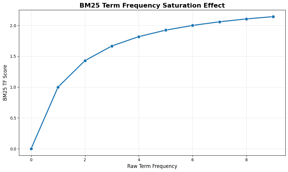
2. Term Frequency Saturation

In basic TF-IDF, a document with 100 mentions of a term gets 10x the score of one with 10 mentions. This can lead to keyword stuffing and poor results. BM25 uses diminishing returns—additional occurrences matter less and less:

def bm25_tf(term_freq, k1=1.5):
    """Calculate BM25 term frequency with saturation."""
    return (term_freq * (k1 + 1)) / (term_freq + k1)

With k1=1.5, the progression looks like:

• 1 occurrence → score of 1.0
• 2 occurrences → score of 1.4 (not 2.0)
• 10 occurrences → score of 2.2 (not 10.0)

This prevents any single term from dominating the results. We can visualize this diminishing return by plotting the term frequency with saturation at different frequencies.

3. Document Length Normalization

Long documents mention more words, boosting their scores unfairly. A 1000-word article about "kubernetes" will naturally contain more search terms than a focused 100-word guide—but that doesn't make it more relevant.

BM25 fixes this with length normalization. Documents longer than average get penalized. Shorter ones get boosted:

import numpy as np

# Calculate mean document length
doc_lengths = [len(process_text(doc)) for doc in documents.values()]
avg_doc_length = np.mean(doc_lengths)

print(f"Document lengths: {doc_lengths}")
print(f"Mean document length: {avg_doc_length:.1f} tokens")

Document lengths: [13, 8, 9, 9]
Mean document length: 9.8 tokens

def length_normalization(document, avg_doc_length=avg_doc_length, b=0.75):
    doc_length = len(process_text(document))
    return 1 - b + b * (doc_length / avg_doc_length)

# Length penalty formula
length_normalization('A short document')

np.float64(0.40384615384615385)

length_normalization('A much longer document with a lot more words in it so it is longer than the average document!')

np.float64(1.403846153846154)

The plot shows this in action. At average length, there's no penalty. Longer documents get increasingly penalized, while shorter ones get boosted.

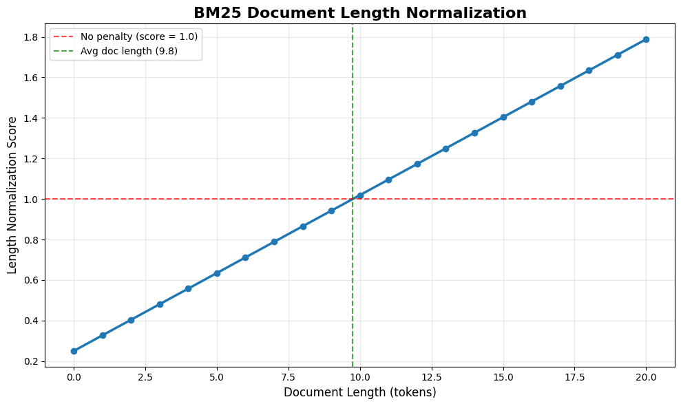
At 0 tokens: 0.250
At avg length (9.8): 1.000
At 20 tokens: 1.788

Full BM25

Now we can put it all together

def bm25_score(term, document_tokens, all_document_tokens, k1=1.5, b=0.75):
    """Calculate complete BM25 score for a term in a document."""
    # Term frequency with saturation
    tf = document_tokens.count(term)
    tf_component = (tf * (k1 + 1)) / (tf + k1)
    
    # Inverse document frequency
    N = len(all_document_tokens)
    df = sum(1 for doc in all_document_tokens if term in doc)
    idf = math.log((N - df + 0.5) / (df + 0.5) + 1)
    
    # Length normalization
    doc_length = len(document_tokens)
    avg_doc_length = sum(len(doc) for doc in all_document_tokens) / len(all_document_tokens)
    length_norm = 1 - b + b * (doc_length / avg_doc_length)
    
    # Apply length normalization to TF
    tf_normalized = (tf * (k1 + 1)) / (tf + k1 * length_norm)
    
    return idf * tf_normalized

To score a document, we calculate the bm25_score for every term in the user query and sum them up

def bm25_document_score(query_terms, document_tokens, all_document_tokens):
    """Calculate total BM25 score for a document."""
    score = 0
    for term in query_terms:
        score += bm25_score(term, document_tokens, all_document_tokens)
    return score

# Score documents for "machine learning"
user_query = "machine learning"
query = process_text(user_query)
print(f"BM25 scores for '{user_query}':")

for doc_id, text in documents.items():
    doc_tokens = process_text(text)
    score = bm25_document_score(query, doc_tokens, all_doc_tokens)
    print(f"Document {doc_id}: {score:.2f} : {text}")

BM25 scores for 'machine learning':
Document 1: 0.92 : Machine learning algorithms are essential for data science. Machine learning models require training data.
Document 2: 0.78 : Python programming supports machine learning libraries like scikit-learn.
Document 3: 0.74 : Data science involves statistics and machine learning techniques for analysis and visualization.
Document 4: 0.00 : Web development with Python uses frameworks like Django and Flask.

This gives us the complete BM25 algorithm: term frequency with saturation, stable IDF calculation, and length normalization all working together to produce relevance scores that match human intuition about what makes a good search result.

Putting It All Together

We've built a complete keyword search system from the ground up, progressing from basic text processing to sophisticated ranking algorithms. Here's how all the pieces fit together:

1. Text Processing: Clean and normalize text for consistent matching
2. Tokenization: Break text into searchable terms while removing noise
3. Inverted Index: Enable fast lookups instead of slow document scans
4. Boolean Operations: Give users precise control over term combinations
5. TF-IDF Scoring: Rank results by relevance using frequency and rarity
6. BM25 Improvements: Provide more robust scoring when dealing with real-world problems

The result is a search system that's both fast and intelligent—capable of finding relevant results in milliseconds.

Learning More